# Load Packages
library(tidyverse) |> suppressPackageStartupMessages()
library(knitr)
library(survival)
library(ggsurvfit)
library(survminer) |> suppressPackageStartupMessages()
library(gt)2 Kaplan Meier
2.1 Kaplan Meier Survival Estimate
The Kaplan Meier survival estimate is how survival probabilities can be calculated while factoring in censored times. The Kaplan Meier survival estimate is used to calculate probability of survival at a given time where \(S(t_j)\) is the probability of being alive at time \(t_j\), \(S(t_{j-1})\) is the probability of being alive at \(t_{j-1}\), \(n_j\) is the number of patients alive just before \(t_j\), \(d_j\) is the number of events at \(t_j\), and \(j\) is the time interval of interest. The equation is \(S(t_j)=S(t_{j-1})(1-\frac{d_j}{n_j})\) (Clark (2003)). The equation essentially divides the surviving individuals by the individuals at risk, similar to the previous calculations shown. However, Kaplan Meier curves adjust for right-censored times by dropping observations from the total number of individuals at risk, \(n_j\), after their censored time has been reached. This adjustment prevents overestimating the survival probability because it no longer assumes censored individuals are still alive or and at risk (Goel (2010)).
2.2 Descriptive Statistics and the Kaplan Meier Curve
Summary statistics can be used to understand Kaplan Meier survival estimates. For example, a 95% confidence interval for the survival probability can be found for each time in the data set using the formula \(S(t_j) ± 1.96 * SE(S(t_j))\) (Sullivan (2016b)). This interval will output a range that, with 95% confidence, contains the true survival probability for an individual in the data set at that time. Another commonly reported descriptive statistic is the median of the survival function, \(S(t_j)\). The median value is the time \(t\) at which \(S(t_j) = 0.5\), or when half of the individuals have not yet experienced the outcome (Rao (2023)).
The Kaplan Meier curve is a graphical representation of the survival function. Similar to the survival probabilities discussed in Section 1.2, the Kaplan Meier curve shows the relationships between time, which is typically plotted on the x-axis, and probability of survival, which is typically on the y-axis. The curve always ranges from 0 to 1 and is typically right skewed.
2.3 Kaplan Meier in R
Luckily, modern software makes these calculations easy and fast, as well as plotting them with confidence intervals and risk tables. A new data set with censored times will be created to demonstrate this process. To do this, a 0 will be recorded for some individuals at times before t = 10. Table 2.1 shows this data set’s structure.
# Create data set
id <- c(1, 2, 3, 4, 5, 6, 7, 8, 9, 10)
time <- c(1, 2, 10, 4, 5, 6, 10, 8, 9, 10)
status <- c(1, 1, 0, 0, 1, 0, 0, 1, 1, 0)
censor <- data.frame(id, time, status)
censor %>% gt(caption = "Example Data Set with Censored Times") %>%
cols_label(id = "ID", time = "Time", status = "Status") | ID | Time | Status |
|---|---|---|
| 1 | 1 | 1 |
| 2 | 2 | 1 |
| 3 | 10 | 0 |
| 4 | 4 | 0 |
| 5 | 5 | 1 |
| 6 | 6 | 0 |
| 7 | 10 | 0 |
| 8 | 8 | 1 |
| 9 | 9 | 1 |
| 10 | 10 | 0 |
The survival package in R has a function called Surv() that takes input data and creates a response object recording survival time for each observation. The function takes in the time variable and the status variable. The function takes into account right censoring as well, marking censored times with a \(+\) symbol in the object created (Zabor (2023)).
# Show the time of event or censored time for each observation
times <- Surv(censor$time, censor$status)
times
[1] 1 2 10+ 4+ 5 6+ 10+ 8 9 10+The survfit() function can be used to calculate the Kaplan Meier survival estimate for each time that a new event occurs. The function takes in the response object created by the Surv() function in order to drop censored observations from the regression. We use ‘times ~ 1’ because we are not including predictor variables in the model. The function returns a survival object that can be used to plot the Kaplan Meier curve and calculate summary statistics. The time variable in the object created by the survfit() function shows the time of each event, and the surv variable shows the survival probability for the remaining individuals after each event occurs.
# Calculate survival object
s1 <- survfit(times ~ 1, data = censor)
# View the survival time for each time an event occurs
s1$time
[1] 1 2 4 5 6 8 9 10# View survival probability for remaining individuals after each event occurs
round(s1$surv, 2)[1] 0.90 0.80 0.80 0.69 0.69 0.55 0.41 0.41The ggsurvfit package can be used to plot the Kaplan Meier curve for this data using the previously created s1 object. Figure 2.1 shows the Kaplan Meier curve for predicting the event. The risk table shows the number of individuals at risk at each time point and the number of events that occurred at each time point.
s1 %>%
  ggsurvfit() +
  labs(
    x = "Time",
    y = "Overall survival probability",
    title = "Kaplan Meier Survival Curve"
  ) +
  scale_x_continuous(breaks=seq(0,10,by=2)) +
  scale_y_continuous(breaks=seq(0,1,by=.2)) +
  add_risktable()
2.4 Log-Rank Test
One of the most common applications of survival analysis and Kaplan Meier curves is for comparing survival times between two groups. One example of when this might be useful is if a study is comparing survival after two different treatment plans. A data set with two groups will be created to demonstrate this process.
# Create new data set
time <- c(8, 7, 10, 8, 5, 3, 4, 10, 6, 1)
status <- c(0, 1, 0, 1, 0, 1, 0, 0, 1, 1)
group <- c(1, 1, 1, 1, 1, 2, 2 ,2, 2, 2)
surv2 <- data.frame(time, status, group)
To run an analysis, the statistical test called the Log-Rank Test can be used to test the null hypothesis that there is no difference between the survival estimates of two groups at any point in time (Rich (2010)). The test is conducted by comparing the observed number of events with an estimated number of events for each group at each time. To calculate expected number of events, the assumption that the two curves are identical is used. The expected number of events at a time \(t\) is for group \(i\) calculated by the formula \(E_{it} = \frac{N_{it} \times O_{t}}{N_{t}}\), where \(N_{it}\) is the observed number of events in group \(i\) at time \(t\), \(O_{t}\) is the total number of events in all groups at time \(t\), and \(N_{t}\) is the total number observations at risk in all groups at time \(t\) (Sullivan (2016a)). Table 2.2 shows the creation of all of these values. The following variables are in the table:
- \(Time\): time when the event occurs
- \(N_{1t}\): the number of people alive and still in the study (at risk), at time \(t\) in group 1
- \(N_{2t}\): the number at risk at time \(t\) in group 2
- \(N_t\): the total number of people at risk in the study at time \(t\)
- \(O_{1t}\): the number of observed events occurring at time \(t\) in group 1
- \(O_{2t}\): the number of observed events occurring at time \(t\) in group 2
- \(O_t\): the total observed events across both groups at time t
- \(E_{1t}\): the expected number of events at time \(t\) in group 1
- \(E_{2t}\): the expected number of events at time \(t\) in group 2
- \(Et\): the total expected number of events across both groups at time \(t\)
Time <- c(1, 3, 4, 5, 6, 7, 8, 10)
N1t <- c(5, 5, 5, 5, 4, 4, 3, 1)
N2t <- c(5, 4, 3, 2, 2, 1, 1, 1)
O1t <- c(0, 0, 0, 0, 0, 1, 1, 0)
O2t <- c(1, 1, 0, 0, 1, 0, 0, 0)

log_rank <- data.frame(Time, N1t, N2t, O1t, O2t)

# Calculate Totals
log_rank$Nt <- log_rank$N1t + log_rank$N2t
log_rank$Ot <- log_rank$O1t + log_rank$O2t
log_rank$E1t <- (log_rank$N1t * log_rank$Ot) / log_rank$Nt
log_rank$E2t <- (log_rank$N2t * log_rank$Ot) / log_rank$Nt

round(log_rank, 2) %>%
  gt() %>%
tab_header("Values Needed to Calculate Chi-Square Statistic")| Values Needed to Calculate Chi-Square Statistic | ||||||||
| Time | N1t | N2t | O1t | O2t | Nt | Ot | E1t | E2t |
|---|---|---|---|---|---|---|---|---|
| 1 | 5 | 5 | 0 | 1 | 10 | 1 | 0.50 | 0.50 |
| 3 | 5 | 4 | 0 | 1 | 9 | 1 | 0.56 | 0.44 |
| 4 | 5 | 3 | 0 | 0 | 8 | 0 | 0.00 | 0.00 |
| 5 | 5 | 2 | 0 | 0 | 7 | 0 | 0.00 | 0.00 |
| 6 | 4 | 2 | 0 | 1 | 6 | 1 | 0.67 | 0.33 |
| 7 | 4 | 1 | 1 | 0 | 5 | 1 | 0.80 | 0.20 |
| 8 | 3 | 1 | 1 | 0 | 4 | 1 | 0.75 | 0.25 |
| 10 | 1 | 1 | 0 | 0 | 2 | 0 | 0.00 | 0.00 |
To test the null hypothesis that there is no difference between the survival estimates of two groups at any point in time, a test statistics is needed. For the Log-Rank test, a Chi-Square test statistic is used because the data follows a Chi-Square curve rather than a normal distribution. The Chi-Square test statistic is calculated by the formula \(X^2 = \sum_{i=1}^k \frac{(\sum{O_{it}} - \sum{E_{it}})^2}{\sum{Vi}}\), where \(\sum_{0}^T{O_{it}}\) is the sum of the observed number of events in group \(i\) over the entire time interval and \(\sum_{0}^T{E_{it}}\) is the sum of the expected number of events in group \(i\) over the entire time interval. The difference of the sums of these two values are divided by the sum of the variance. The variance for group 1 at time \(t\) is calculated by the formula \(V_{1t} = \frac{N_{1t} \times N_{2t} \times O_{t} \times (N_{t} - O_{t})}{N_{t}^2 \times (N_{t} - 1)}\) (Collet (2003)). The variance for group 2 is calculated similarly, and the total variance is calculated by the formula \(V_{t} = V_{1t} + V_{2t}\). Table 2.3 shows the calculation of the Chi-Square test statistic for the data set. Two new variables are calculated from the previous table:
- \(V_{1t}\): the variance of the number of events at time \(t\) in group 1
- \(V_{2t}\): the variance of the number of events at time \(t\) in group 2
log_rank$V1t <- (log_rank$N1t * log_rank$N2t * log_rank$Ot *
                   (log_rank$Nt - log_rank$Ot)) /
  (log_rank$Nt^2 * (log_rank$Nt - 1))

log_rank$V2t <- (log_rank$N1t * log_rank$N2t * log_rank$Ot *
                   (log_rank$Nt - log_rank$Ot)) /
  (log_rank$Nt^2 * (log_rank$Nt - 1))

round(log_rank, 2) %>%
  gt() %>%
tab_header("Calculation of Variance")| Calculation of Variance | ||||||||||
| Time | N1t | N2t | O1t | O2t | Nt | Ot | E1t | E2t | V1t | V2t |
|---|---|---|---|---|---|---|---|---|---|---|
| 1 | 5 | 5 | 0 | 1 | 10 | 1 | 0.50 | 0.50 | 0.25 | 0.25 |
| 3 | 5 | 4 | 0 | 1 | 9 | 1 | 0.56 | 0.44 | 0.25 | 0.25 |
| 4 | 5 | 3 | 0 | 0 | 8 | 0 | 0.00 | 0.00 | 0.00 | 0.00 |
| 5 | 5 | 2 | 0 | 0 | 7 | 0 | 0.00 | 0.00 | 0.00 | 0.00 |
| 6 | 4 | 2 | 0 | 1 | 6 | 1 | 0.67 | 0.33 | 0.22 | 0.22 |
| 7 | 4 | 1 | 1 | 0 | 5 | 1 | 0.80 | 0.20 | 0.16 | 0.16 |
| 8 | 3 | 1 | 1 | 0 | 4 | 1 | 0.75 | 0.25 | 0.19 | 0.19 |
| 10 | 1 | 1 | 0 | 0 | 2 | 0 | 0.00 | 0.00 | 0.00 | 0.00 |
For group 1 at time 1, we would calculate \(E_{1t} = \frac{5 \times 1}{10} = 0.50\) and for group 2 at time 1, \(E_{2t} = \frac{5 \times 1}{10} = 0.50\). We would repeat for each group at each time and then sum the values to get \(\sum_{t=1}^t{E_{i}}\) for each group. For group 1, \(\sum_{t=1}^t{E_{1}} = 0.50 + 0.56 + 0 + 0 + 0.67 + 0.80 + 0.75 + 0 = 3.27\) and for group 2, \(\sum_{t=0}^t{E_{2}} = 0.50 + 0.44 + 0 + 0 + 0.33 + 0.20 + 0.25 + 0 = 1.73\). The sum of the observed events for group 1 is 2 and for group 2 is 3. For group 1 at time 1, we would calculate \(V_1t = \frac{5 \times 5 \times 1 \times (10-1)}{10^2 \times (10-1)} = 0.25\) Table 2.4 shows the rest of the variances calculated for both groups for the surv2 data set. The table includes the following new variables:
- \(SumO_{1t}\): the sum of the observed number of events in group 1 over the entire time interval
- \(SumO_{2t}\): the sum of the observed number of events in group 2 over the entire time interval
- \(SumE_{1t}\): the sum of the expected number of events in group 1 over the entire time interval
- \(SumE_{2t}\): the sum of the expected number of events in group 2 over the entire time interval
- \(SumV_{1t}\): the sum of the variance of the number of events at time \(t\) in group 1
- \(SumV_{2t}\): the sum of the variance of the number of events at time \(t\) in group 2
- \(X_1\): the Chi-Square test statistic for group 1
- \(X_2\): the Chi-Square test statistic for group 2
SumO1t <- cumsum(log_rank$O1t)
SumO2t <- cumsum(log_rank$O2t)
SumE1t <- cumsum(log_rank$E1t)
SumE2t <- cumsum(log_rank$E2t)
SumV1t <- cumsum(log_rank$V1t)
SumV2t <- cumsum(log_rank$V2t)

# Create table with each of the last values
sum_stats <- data.frame(SumO1t, SumO2t,
                        SumE1t, SumE2t, SumV1t, SumV2t)
# Get the last row of summary statistics
sum_stats <- sum_stats[nrow(sum_stats), ]
sum_stats$X1 <- ((sum_stats$SumO1t - sum_stats$SumE1t)^2 /
                          sum_stats$SumV1t)
sum_stats$X2 <- ((sum_stats$SumO2t - sum_stats$SumE2t)^2 /
                          sum_stats$SumV2t)

round(sum_stats, 2) %>%
  gt() %>%
tab_header("Calculation of Chi Square Statistic")| Calculation of Chi Square Statistic | |||||||
| SumO1t | SumO2t | SumE1t | SumE2t | SumV1t | SumV2t | X1 | X2 |
|---|---|---|---|---|---|---|---|
| 2 | 3 | 3.27 | 1.73 | 1.07 | 1.07 | 1.52 | 1.52 |
With all of these values, we can calculate the Chi Square test statistic, \(X^2_i = \frac{(\sum{O_{it}} - \sum{E_{it}})^2}{V_{it}}\). We get \(X^2_{1} = \frac{(2 - 3.27)^2}{1.07} = 1.51\) and \(X^2_2 = \frac{(3 - 1.73)^2}{1.07} = 1.51\). The test statistic can then be compared to a Chi-Square distribution with one \(k-1\) degrees of freedom, with \(k\) being the number of groups. So, for this example, \(k\) is 2 and there is 1 degree of freedom (Sullivan (2016a)).
Clearly, calculating the test statistic is very tedious, even for a data set with 10 observations. The survdiff function can be used to run a Log-Rank test in R, making it much easier to run the test. The function takes in the response object created by the Surv() function and the grouping variable (Zabor (2023)). It returns a Chi-Square statistic and a p-value. We can see that the p-value is much higher than 0.05, indicating that we do not have evidence to reject the null hypothesis, and thus that there is no difference between the survival estimates of the two groups.
# Calculate times for events in this data set
times2 <- Surv(surv2$time, surv2$status)
# Run a log rank test based on group variable
test_stat <- survdiff(times2 ~ group, data = surv2)
test_stat
Call:
survdiff(formula = times2 ~ group, data = surv2)
N Observed Expected (O-E)^2/E (O-E)^2/V
group=1 5 2 3.27 0.495 1.52
group=2 5 3 1.73 0.937 1.52
Chisq= 1.5 on 1 degrees of freedom, p= 0.2 The only adjustment needed for plotting the Kaplan Meier curves for two groups is to include the grouping variable while making the survival object using the survfit function (Zabor (2023)). The two survival curves are depicted in Figure 2.2.
# Create survival object using group as a predictor
s2 <- survfit(Surv(time, status) ~ group, data = surv2)

# Plot the two curves
s2 %>%
  ggsurvfit() +
  labs(
    x = "Days",
    y = "Overall survival probability",
    title = "Kaplan Meier Survival Curve by Group"
  ) +
  scale_x_continuous(breaks=seq(0,10,by=2)) +
  scale_y_continuous(breaks=seq(0,1,by=.2)) +
  add_risktable()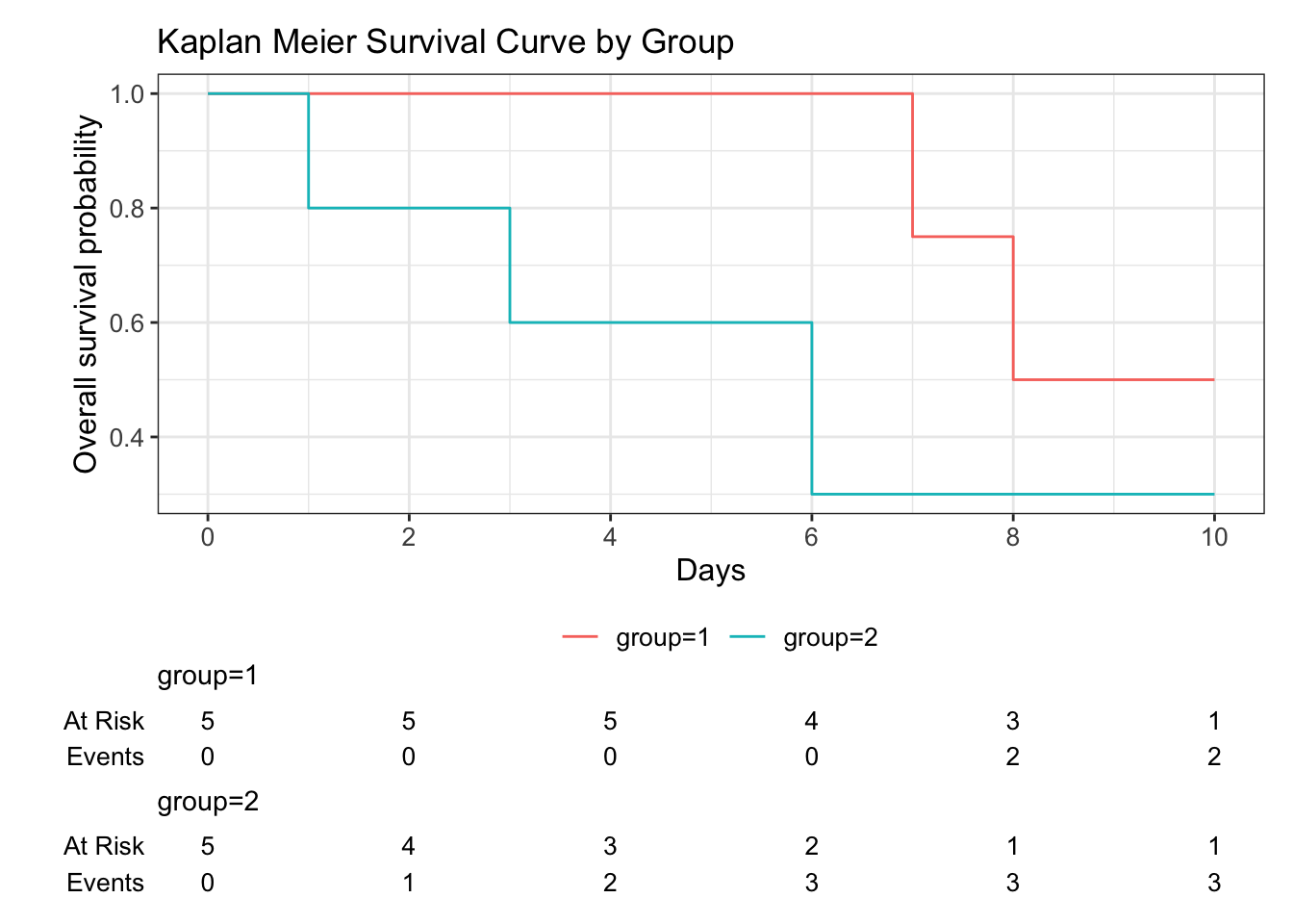
2.5 Case Study: Cirrhosis Data
The next example uses a data set with variables for predicting death in patients with cirrhosis, which is permanent scarring of the liver. The data set is from a clinical trial conducted by the Mayo Clinic from 1974 to 1984. The data set contains 424 primary biliary cirrhosis patients with 20 variables (Fedesoriano (2021)). To conduct survival analysis, the Status variable needs to be transformed into an indicator variable, labelled event, coded as a 1 representing death and 0 representing censored. The N_Days variable will be used for the time variable, indicating number of days since the beginning of the trial.
cirrhosis <- read_csv("data/cirrhosis.csv", show_col_types = FALSE)
cirrhosis <- cirrhosis %>% mutate(event = if_else(Status == 'D', 1, 0))
The main interest of this data is to explore the difference in survival time between patients taking the drug of interest, D-penicillamine, and those given a placebo. The variable Drug indicates which group the patient was in and will be used as the grouping variable for a Log-Rank Test. Below, we calculate an object with times of event for this data and then use the survdiff function to run a Log-Rank Test.
# Calculate times and store in an object
times3 <- Surv(cirrhosis$N_Days, cirrhosis$event)

# Run a log rank test based on drug group
survdiff(times3 ~ Drug, data = cirrhosis)
Call:
survdiff(formula = times3 ~ Drug, data = cirrhosis)
n=312, 106 observations deleted due to missingness.
N Observed Expected (O-E)^2/E (O-E)^2/V
Drug=D-penicillamine 158 65 63.2 0.0502 0.102
Drug=Placebo 154 60 61.8 0.0513 0.102
Chisq= 0.1 on 1 degrees of freedom, p= 0.7 From the Log-Rank test, we see that the p-value is 0.7, which is much larger than 0.05. This indicates that the test was not statistically significant at the five percent level. Thus, there was no statistically significant difference between patient outcome between the two treatment groups. So, for patients with biliary cirrhosis, we did not find evidence that D-penicillamine is an effective drug for preventing death.
We can visualize this in Figure 2.3, which shows the survival curves for both groups of patients. We can also use the ggsurvplot function from the survminer() package to plot the survival curves. The curves are very similar and cross multiple times, which makes sense since we know the drug of interest did not have a significant effect on patient survival.
# Create Survival Object
s3 <- survfit(times3 ~ Drug, data = cirrhosis)

# Plot the survival curves
s3 %>% ggsurvplot(
    palette = c("darkgreen", "maroon"),
    legend.labs = c("D-penicillamine", "Placebo"),
    xlab = "Time",
    ylab = "Survival Probability",
    title = "Kaplan Meier Survival Curve by Drug Group"
  )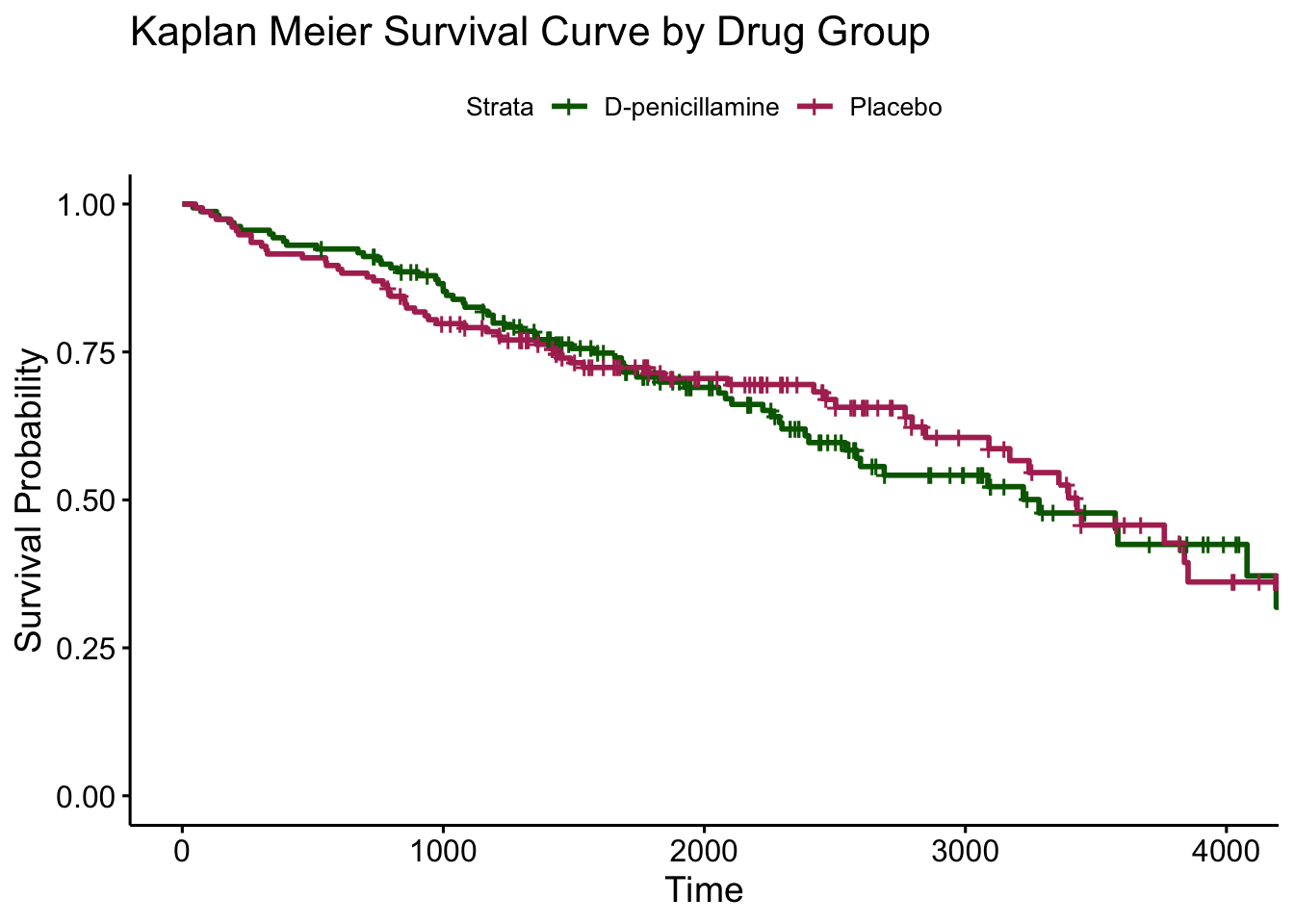
As we can see, the two survival curves are very similar and cross multiple times, which makes sense since we know the drug of interest did not have a significant effect on patient survival.
2.6 Case Study: Heart Failure Data
Let’s look at another data set which contains information on patients with heart failure. The data set contains data on heart failure patients over 40 years old who were admitted to the Institute of Cardiology at the Allied hospital Faisalabad-Pakistan between April and December of 2015. All of the patients in the data set had left ventricular systolic dysfunction and belonged to NYHA class III and IV stages of heart failure (Ahmad (2017)).
heart <- read_csv("data/S1Data.csv") Rows: 299 Columns: 13
── Column specification ────────────────────────────────────────────────────────
Delimiter: ","
dbl (13): TIME, Event, Gender, Smoking, Diabetes, BP, Anaemia, Age, Ejection...
ℹ Use `spec()` to retrieve the full column specification for this data.
ℹ Specify the column types or set `show_col_types = FALSE` to quiet this message.Let’s view the Kaplan Meier survival curves to see if there is a visual difference in survival probabilities for individuals with normal versus high blood pressure. In this data set, blood pressure is a binary variable where 0 indicates normal blood pressure and 1 indicates high blood pressure. It is called BP in the data set. We can view the curve in Figure 2.4.
# Create Survival Object
times_heart <- Surv(heart$TIME, heart$Event)

# Plot the curves
survfit(times_heart ~ BP, data = heart) %>%
  ggsurvplot(
    palette = c("darkgreen", "maroon"),
    legend.labs = c("Normal BP", "High BP"),
    xlab = "Time (Days)",
    ylab = "Survival Probability",
    title = "Kaplan Meier Survival Curve by Blood Pressure"
  )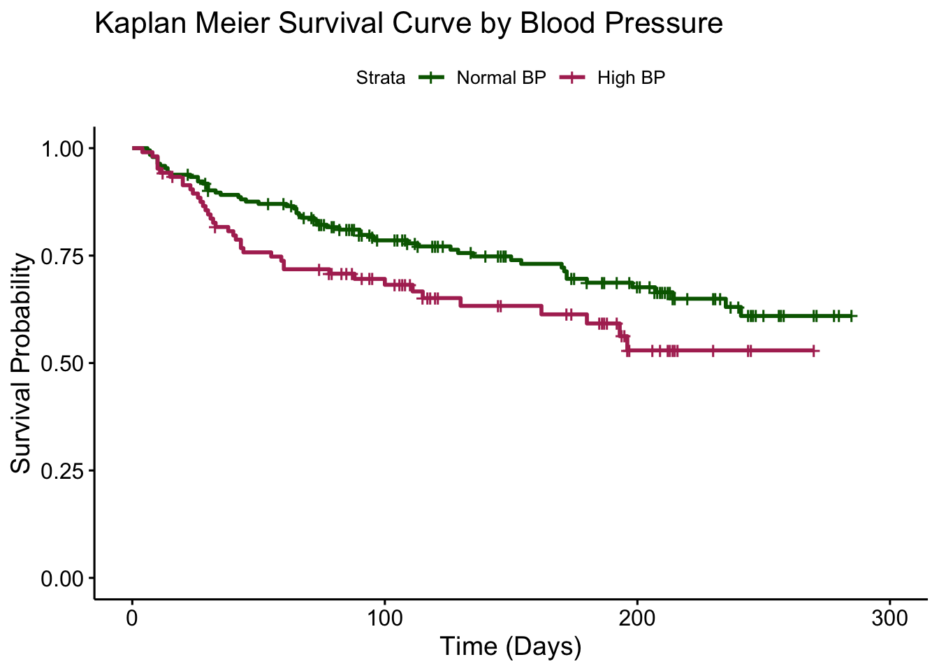
From the curves, it seems like there will be a difference in survival probabilities between individuals with normal and high blood pressure based on the two curves. Let’s run a Log-Rank test to see if the difference is statistically significant.
# Run a log rank test based on blood pressure group
survdiff(times_heart ~ BP, data = heart)
Call:
survdiff(formula = times_heart ~ BP, data = heart)
N Observed Expected (O-E)^2/E (O-E)^2/V
BP=0 194 57 66.4 1.34 4.41
BP=1 105 39 29.6 3.00 4.41
Chisq= 4.4 on 1 degrees of freedom, p= 0.04 The p-value from the Log-Rank test is 0.04, so we can conclude that blood pressure is a significant predictor of survival probability in heart failure patients.
2.7 Limitations
It is important to note the limitations of this analysis. First, the Kaplan Meier function does not allow for the use of continuous variables or multiple predictors in the model. Instead, it is limited to one categorical predictor, such as blood pressure in our cirrhosis model. Additionally, the Log-Rank test only tells us whether there is a difference in survival probabilities, but it does not tell us how big this difference is. So, to gain more understanding on how big the effect of blood pressure is on patient survival, we would need to use other methods of analysis. The next section will discuss other methods that can be used for creating more complex models and learning more about how much of an effect the predictors have on survival.
2.8 References
Ahmad, Munir, T. 2017. “Survival Analysis of Heart Failure Patients: A Case Study.” PLOS ONE 12 (7). https://doi.org/10.1371/journal.pone.0181001.
Clark, Bradburn, T. G. 2003. “Survival Analysis Part i: Basic Concepts and First Analyses.” British Journal of Cancer, May. https://www.ncbi.nlm.nih.gov/pmc/articles/PMC2394262/.
Collet, David. 2003. Modelling Survival Data in Medical Research. Chapman & Hall/CRC.
Fedesoriano. 2021. “Cirrhosis Prediction Dataset.” www.kaggle.com/datasets/fedesoriano/cirrhosis-prediction-dataset/data.
Goel, Khanna, M. K. 2010. “Understanding Survival Analysis: Kaplan-Meier Estimate.” International Journal of Ayurveda Research. https://www.ncbi.nlm.nih.gov/pmc/articles/PMC3059453.
Rao, & Schoenfeld, S. R. 2023. “Statistical Primer for Cardiovascular Research.” AHA Journals. https://www.ahajournals.org/doi/pdf/10.1161/circulationaha.106.614859.
Rich, Neely, J. T. 2010. “A Practical Guide to Understanding Kaplan-Meier Curves.” Otolaryngology–Head and Neck Surgery: Official Journal of American Academy of Otolaryngology-Head and Neck Surgery. https://www.ncbi.nlm.nih.gov/pmc/articles/PMC3932959/.
Sullivan, LaMorte, L. 2016a. “Comparing Survival Curves.” sphweb.bumc.bu.edu/otlt/mph-modules/bs/bs704_survival/BS704_Survival5.html.
———. 2016b. “Estimating the Survival Function.” https://sphweb.bumc.bu.edu/otlt/mph-modules/bs/bs704_survival/bs704_survival4.html.
Zabor, E. C. 2023. “Survival Analysis in r.” https://www.emilyzabor.com/tutorials/survival_analysis_in_r_tutorial.html.